Variance & SD— How far Spreaded !!

Let’s check how spread or dispersed our data is.

Well, we all love to travel for sure. In case you ever traveled from Asian countries to Europe or maybe Asia to any Western countries, have you ever noticed that most connecting flights are from the Middle East ( Dubai or Sharjah mostly )? Why ??

The answer is the variance from the center ( Middle East ) or mean distance from these countries is less.

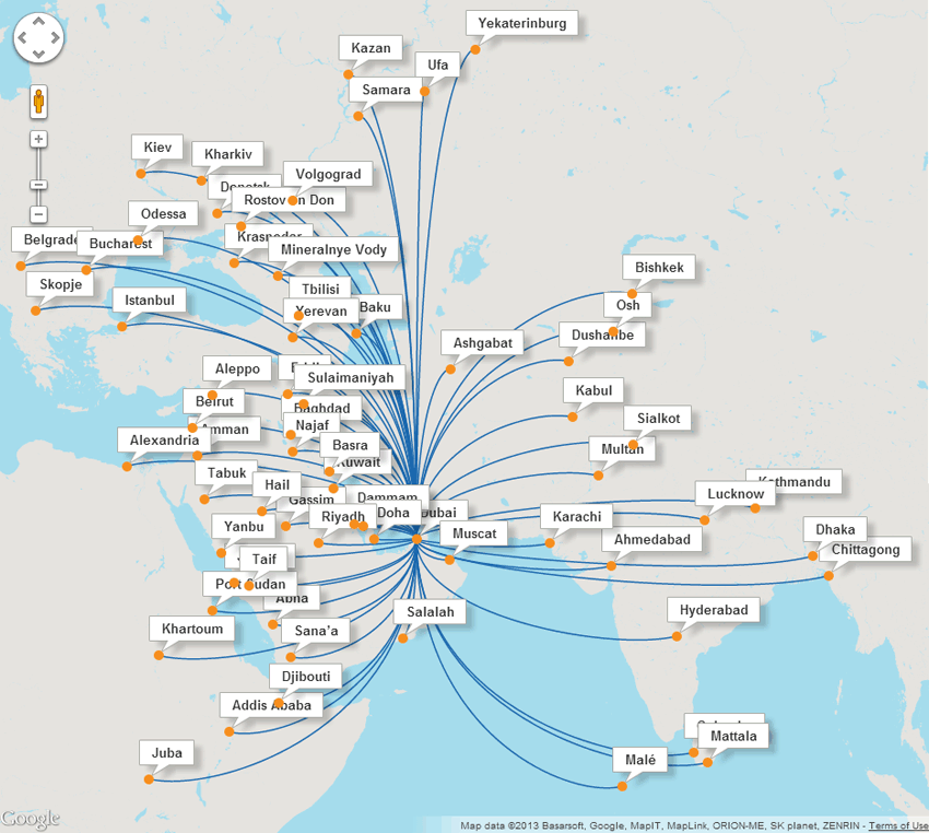
Holds for Paris as well 😁

For more read Hub-and-Spoke Model which reduces the overall variance.

But let’s take one step back and see why we need the variance if we have the mean, median, or mode as a great representative of data.

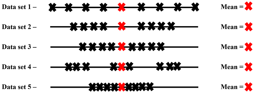
If someone gave you the 1-number summary (central tendency) of the below shown five datasets, in your mind, you would have thought they all are the same since their means are the same but when you plot each data point of each set and compare them visually you will realize that there should exist a measure to detect this distinguishing pattern as well.

Say “Hi” to the spread measure — Variance & Standard Deviation

What is a Variance — Degree of Spread

Variance is a numerical value that shows how widely the individual figures in a data distribution themselves about the mean and hence describes the difference of each value in the dataset from the mean value.

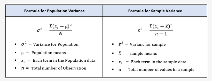
The formula of Variance:-

**Population Variance Formula — Variance is often depicted by this symbol: σ2**

The average of the squared differences from the mean.

Why the numerator is Squared in Variance?

Because, if you didn’t Square the Terms, the opposite signs of (+ve and -ve) values cancel each other and hence it tends to zero. To avoid this, we are squaring the values and hence the values become (+ve).

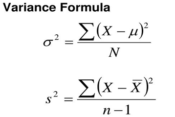
Now, Wait . . . Wait . . . Have you noticed the Sample Variance Formula? there is a slight change in the denominator right when compared to Population variance. . .

Why the denominator (n-1) in Sample Variance?

There are two perspectives:-

Bessel’s correction.

The Sample Variance, s², is used to calculate how varied a sample is,
and it’s useful to estimate the Population Variance. ( Sample Statistics — We find some inferences from the sample and then expand it for the population )

Since the Sample Variance is a kind of estimation, its formula is a bit different.

Assume a case that the sample we took fails to represent the inconsistency of the population. In other words, if the data is skewed our sample will fail to explain the trends of population.

Consider the following example.

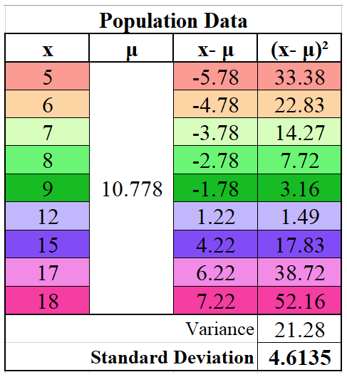
Now we take a subset of the above data and try to calculate the variance by dividing it with “n” (biased) and again with “n-1” (unbiased).

In one shot the reason for using n−1 instead of n in the sample variance formula is to correct for the bias in the estimation of the population variance. This correction is known as Bessel’s correction, named after German mathematician Friedrich Bessel.

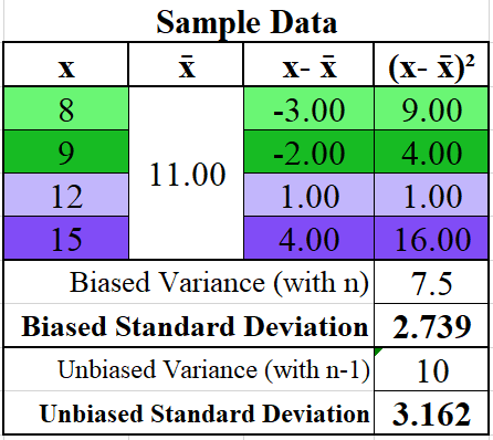
If 10 ( Unbiased Sample variance ) or 7.5 ( Biased Sample variance ) is closer to 21.28 ( Population variance ), you know the answer 😁.

Therefore, to take account of that, we divide by n-1 instead of n which in turn decreases the denominator and increases the variance and additionally acknowledges that one degree of freedom is “lost” when estimating the sample mean ˉxˉ.

2 . Degree of Freedom

If we know the Sample Mean, we can calculate the other data points using the sample mean. When it comes to population, every data point gives an independent and unchanged mean.

Degree of Freedom says that, the minimum number of data points/samples required to calculate the statistic. So, according to this point (If we know the Sample Mean, we can calculate the other data points using the sample mean), we are reducing our denominator to (n-1)

Explanation using Example:

Imagine there is a huge garden near your home. As we can’t measure the heights of all plants, we are inferring it with a sample of plants.

Let’s consider the sample consists of 4 plants (4 Degrees of Freedom) discovering it to be 160cm in total, implying a mean height of 40cm for this subset or sample.

Now, the magic unfolds as we delve into the concept of degrees of freedom. We decided to measure each plant individually, systematically removing one degree of freedom with each measurement.

1st Plant (1st Degree of Freedom): Measuring the first plant reveals a height of 35 cm. This implies that the remaining 3 plants must collectively have a total height of 125cm (160cm — 35cm).
2nd Plant (2nd Degree of Freedom): Measuring the second plant reveals a height of 45 cm, and narrows down the possible total height of the remaining 2 plants to 80cm (160cm — 35cm — 45cm).
3rd Plant (3rd Degree of Freedom): Continuing this, Measuring the 3rd plant reveals a height of 50cm, and narrows down the possible total height of the remaining plant to 30cm (160cm — 35cm — 45cm — 50cm)

We can observe that as per the above example, we find the height of all four plants is calculated by measuring the heights of 3 plants only (3 Degrees of freedom), This means that we can automatically know the height of 4th plant even though you have measured only 3.

This means, that if you have measured (n-1) objects then the nth object has no freedom to vary. Therefore, the degree of freedom is only (n-1) and not n.

Hence by using n−1, we are providing a better estimate of the population variance and avoiding this bias.

Why does n-1 work? — Why wouldn’t n-2 or n/3 work?

Empirically n-1 gives the best approximation.

Explanation: — At last, Why do we specifically choose (n-1) and not (n-2) or (n-3)? The answer lies in the essence of degrees of freedom. When (n-1) objects are measured, the remaining object loses its freedom to vary.

If we were to divide by (n-2) or (n-3), we would be making assumptions about the variability of unmeasured objects that might not hold.

Well, to understand it I’d recommend working through the proofs yourself.

If you found anything in this article to be unclear I highly recommend reading through the Wikipedia article on Bessel’s correction.

In Nutshell,

What does variance convey? — Variability

Let’s say, if we have zero variance in a dataset, we can state that all the values in it are identical.

More variance states the more spread of distribution away from the mean, and lower variance states less spread of distribution away from the mean, but the variance can never be negative.

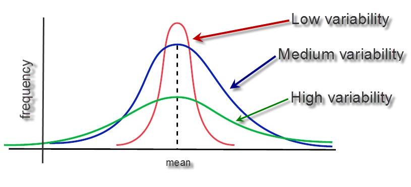
Imagine you’re measuring the heights of students in two different classrooms. If one class has students of similar heights, and the other has students with varying heights, you’d say the second class has higher variability.

You need to know as a data scientist what the implications of variance are in learning your machine.

Two concepts:-

Low Variance:

Definition: Low variance means that the data points in a dataset are very similar to each other.
Implication: When the variance is low, even a small change in the dataset can significantly affect the results or predictions of a model.
Example: If you have a set of exam scores that are all close to 90, introducing a score of 70 will noticeably change the average score.

High Variance:

Definition: High variance indicates that the data points in a dataset are spread out and vary greatly from the mean.
Implication: When the variance is high, only large changes in the dataset will have a noticeable impact on the results or predictions of a model.
Example: If you have a set of exam scores ranging from 50 to 100, changing one score from 60 to 65 won’t significantly affect the average score.

Use cases in Data Science:-

Model performance: In machine learning, variance is used to measure the variability in model performance. High variance can indicate overfitting, where the model performs well on training data but poorly on new data.
Risk Assessment: Variance is used to measure the volatility of asset returns. Higher variance indicates higher risk, as the asset’s returns are more spread out from the mean.

**Average Stock Variance as a Market Indicator**

Suppose an investor is analyzing the returns of two stocks over some time.

Stock A returns: 5%, 7%, 6%, 8%, 7%
Stock B returns: 2%, 10%, 1%, 15%, 3%

Calculating the variance of returns for both stocks:

Stock A: Variance is low, indicating more consistent returns.
Stock B: Variance is high, indicating more volatile returns.

High Variance means high fluctuation from mean or in other words high risk but high chances of returns and low variance means low fluctuation or data is mostly centered around the average stock value with some standard returns.

3. ANOVA

ANOVA (Analysis of Variance) is a statistical method used to compare means across multiple groups and determine if there are any statistically significant differences between them. It is particularly useful in experiments and studies where multiple factors are being tested simultaneously.

For example, Drug Efficacy in Clinical Trials and Medical Research as Anova can be used to compare the effectiveness of different drugs or treatments. For example, comparing the mean recovery times of patients using different medications.

4. Marketing

Customer Satisfaction: Companies analyze the variance in customer satisfaction scores to identify inconsistencies in service or product delivery.
Market Research: Variance is used to understand the diversity of consumer preferences and behaviors, aiding in the development of targeted marketing strategies.

5. Clustering

In machine learning, variance can be used to identify clusters in datasets. Clusters are groups of data points that are similar to one another. Standard deviation and variance allow machine learning algorithms to learn how they differ from each other.

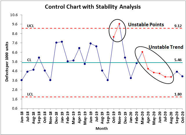
Some more use cases I encountered in my first experience while working as a Quality analyst in manufacturing sector by using control charts

Product Quality: Manufacturers use variance to monitor and control the quality of products. Low variance in product measurements indicates consistency and high quality.
Process Improvement: By analyzing the variance in production processes, companies can identify areas of inefficiency and implement improvements.

What is the Standard deviation?

Standard deviation is a measure of how spread out numbers are in a set of data. It’s used to measure the amount of variation or dispersion from the average of a dataset. In simpler terms, it is the amount of deviation from the mean or average value.

The formula of Standard deviation —

It can be calculated by doing a square root of the variance.

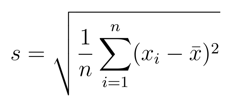
Hang on !! The definition looks similar to variance.

The truth is standard deviation is introduced in statistics due to a disadvantage of the variance which is that the variance calculation gives added weight to the elements that are far from the mean which makes it less accurate. The variance is calculated primarily to take the square root value of it which is the standard deviation.

Same Units as Data:

Variance: Calculated as the average of the squared deviations from the mean, it results in units that are the square of the original data units (e.g., if the data is in meters, the variance is in square meters).
Standard Deviation: The square root of the variance, bringing the units back to the same as the original data (e.g., if the data is in meters, the standard deviation is also in meters). This makes it easier to interpret and understand.

Intuitive Interpretation:

The standard deviation provides a measure of how spread out the data points are around the mean. A smaller standard deviation indicates that the data points are close to the mean, while a larger standard deviation indicates that the data points are more spread out.

Consistency with Normal Distribution:

In the context of the normal distribution (bell curve), the standard deviation is used to describe the spread of data. Approximately 68% of the data falls within one standard deviation of the mean, 95% within two standard deviations, and 99.7% within three standard deviations. This property makes the standard deviation a useful tool for understanding and comparing different datasets.

All in All,

When it comes to units of measurement, the two are stated as follows:

Variance is expressed in squared units (e.g. ounces squared).
Standard deviation is expressed in the same units of measurement as the original units (e.g. ounces).

How is this useful & Intuitive?

Standard deviation is useful because it can tell us where most values lie, what’s a ‘normal’ value, what’s an extreme value, and what’s practically impossible.

In a normal distribution, 1 standard deviation represents about 68% of all values, 2 SDs is 95% of all values, and 3 is 99.7% of all values.

68 -95–99 rule:-

Approximately 68% of all data points fall in the interval μ ± σ (within 1 SD of the mean).
Approximately 95% of all data points fall in the interval μ ± 2σ (within 2 SD of the mean).
Approximately 99.7% of all data points fall in the interval μ ± 3σ (within 3 SD of the mean).

How do high & low Standard Deviations look like:-

The data points are more dispersed, therefore the standard deviation is higher.

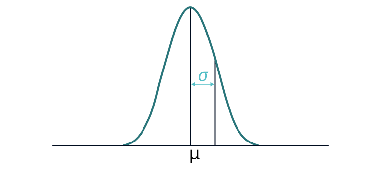
The graph above shows a distribution with observations that are more clustered around the mean, resulting in a lower standard deviation.

In a nutshell, with the 2-number summary (Central Tendency & Spread), we can better distinguish among datasets and remember every statistical measure has a purpose to serve. These measures exist to capture details that were not captured with already available measures like mean and median.

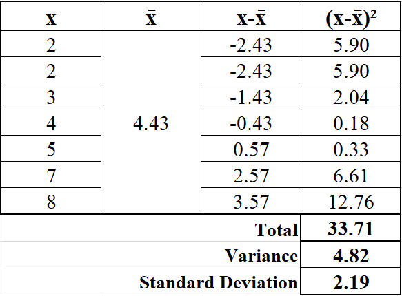
Let’s calculate both step by step:-

Consider the following example. Here there are 7 data points ( n = 7 ) for which the mean is 4.43 and the standard deviation is 2.19. Now if we plot these details and see in a normal distribution we would be able to identify the regions where these points lie and how far the data stretches.

Standard Deviation vs Variance

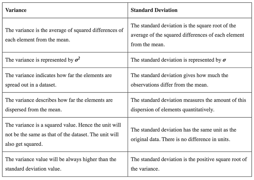
Unlike variance, we measure standard deviation in the same units as the observations. This makes it the preferred method to assess variability, especially regarding practical applications such as data analysis, decision-making, and reporting.

But fortunately,

If the variance is large => the Standard Deviation is also large
If the variance is small => the Standard Deviation is also small

Python Code

import numpy as np
import pandas as pd

# Sample data
data = [10, 12, 23, 23, 16, 23, 21, 16]

# Using numpy
variance_np = np.var(data, ddof=1)  # Sample variance
std_dev_np = np.std(data, ddof=1)  # Sample standard deviation

print("Using numpy:")
print(f"Variance: {variance_np}")
print(f"Standard Deviation: {std_dev_np}")

# Using pandas
data_series = pd.Series(data)
variance_pd = data_series.var()
std_dev_pd = data_series.std()

print("\nUsing pandas:")
print(f"Variance: {variance_pd}")
print(f"Standard Deviation: {std_dev_pd}")