GRADIENT DESCENT — A Journey, not a Destination to reach Global Minima.

What is Gradient Descent?

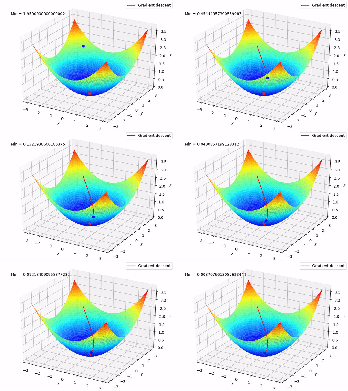
Gradient descent is an iterative machine learning optimization algorithm to reduce the cost function so that we have models that make accurate predictions.

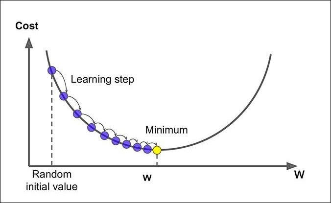
The Goal is minimise the Cost or Loss functions to reach at Global Minima.

Cost function

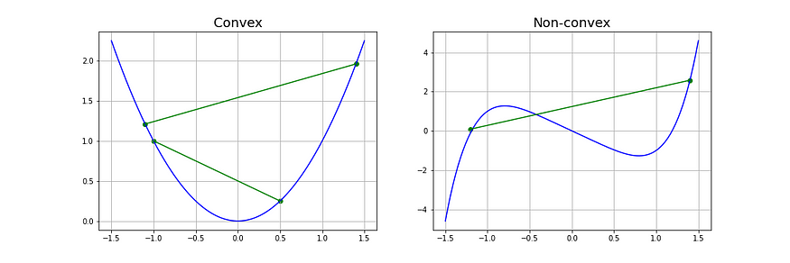
Cost function(C) or Loss function measures the difference between the actual output and predicted output from the model. The cost function is a convex function.

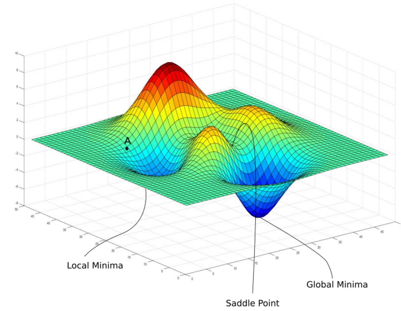
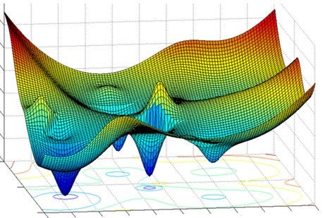
When selecting an optimization algorithm, it is essential to consider whether the loss function is convex or non-convex. A convex loss function has only one global minimum and no local minimum, making it easier to solve with a simpler optimization algorithm. However, a non-convex loss function has both local and global minima and requires an advanced optimization algorithm to find the global minimum.

What Exactly is a Loss Function?

In typical machine learning problems, there is always an input and a desired output. However, the machine doesn’t know that. Instead, the machine uses some of the input that it is given, as well as some of the outputs that are already known to be used in predictions.

Determining the best machine learning model for a certain situation often entails comparing the machine’s predictions and the actual results to determine whether or not the algorithm used is accurate enough.

The problem is, how do we know whether or not the machine is learning effectively? This is where optimization enters the picture in the form of a loss function.

To increase accuracy, the value of the loss function must be at the minimum. An example of a simple loss function is the mean-squared-error (MSE) which is given by the expression below:

Expression for Mean-Squared Error (MSE)

Here, n refers to the number of data points; yi, is the actual output; xi, is the machine’s prediction.

Each iteration and evaluation of the loss function for each data point is called an epoch. ( Iteration ). In a working machine learning model, the loss function decreases with the more epochs it iterates through.

In machine learning, optimization is the process of finding the ideal parameters, or weights, to maximize or minimize a cost or loss function.

The global maximum is the largest value on the domain of the function, whereas the global minimum is the smallest value. While there is only one global maximum and/or minimum, there can be many local maxima and minima.

The global minimum of a cost function indicates where a model’s parameters generate predictions that are close to the actual targets.

The local maxima and minima can cause problems when training a model.

Lets respect the history & Inventors for this Big Bang Theory of ML.

The “gradient descent” algorithm was invented before the gradient and the early inventor was Cauchy a French mathematician in 1847. He described the same in her 3 — Page paper Comptes Rendus, Méthode générale pour la résolution des systèmes d’équations simultanées (1847). Instead of the gradient vector Cauchy simply works with the partial derivatives.

The idea of Gradient Descent in Statistical models dates back to the early 19th century when Carl Friedrich Gauss proposed the method of least squares for fitting a linear model to data. The method of steepest descent, also known as the saddle-point method, is a natural development of Laplace’s method.

Let’s drill down the Gradient Descent in to pieces.

Gradient

A gradient is the vector ( direction and magnitude ) calculated during the training of a model and points in the direction of the steepest descent of a function at a particular point.

In the context of Deep learning, it is used to teach the network weights in the right direction by the right amount.

Let’s understand why we calculate the derivatives:-

Derivative: In one dimension, the derivative of a function represents the rate of change of that function concerning its input variable. By knowing how the function changes as we adjust its parameters, we can determine the direction in which to move to minimize the function.

In the context of Gradient Descent,

Derivatives indicate the direction of the steepest ascent or descent of a function.
Gradient Descent utilizes this information to iteratively update parameters, aiming to minimize or maximize the function.

Geometrically, we can also think of a gradient as the slope of the tangent line to the curve at a given point. The concept of slope is used to measure the rate at which changes are taking place.

Now read the below statement, this will make more sense.

Gradient: In multiple dimensions, a function may have multiple input variables. The gradient of the function is a vector that contains the partial derivatives of the function concerning each of its input variables.

Each component of the gradient represents the rate of change of the function for one of the variables while holding the others constant.

The higher the gradient, the steeper the slope and the faster a model can learn. But if the slope is zero, the model stops learning. Said more mathematically, a gradient is a partial derivative of its inputs.

Let me make you feel more comfortable,

To understand how gradients work, let’s consider a simple example. Suppose we have a function f(x) = x². The gradient of this function concerning x is dx/df = 2x. This gradient tells us how f changes as we vary x. For instance, when x = 2, the gradient is 2 × 2 = 4, indicating that f increases at a rate of 4 units for every unit increase in x.

Descent

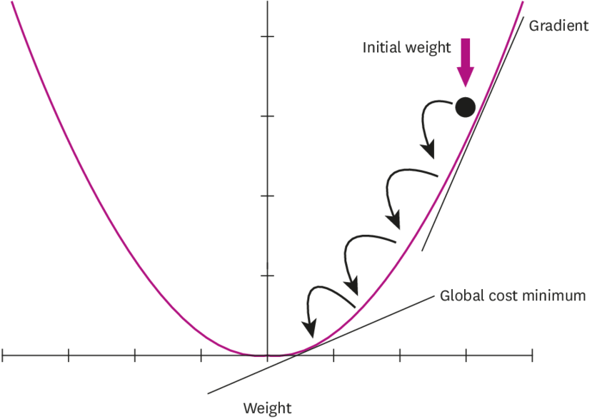
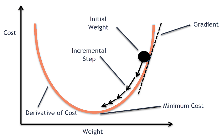
Descent, in simple terms, means going down. Remember, the algorithm goal is to find the lowest point (minimum or Global Minima ) of a cost function where the loss is expected to minimum( Optimised point ). The slope ( gradient ) will guide us at every step to move in the right direction towards Global Minima.

It’s the negative of the gradient points in the direction of the steepest descent, where the function value decreases the most rapidly. Also, remember if you move in the direction of the gradient, the function value will increase the most rapidly. ( Avoiding this situation )By repeatedly moving in the direction opposite to the gradient, the algorithm aims to converge towards a local or global minimum (or maximum) of the function.

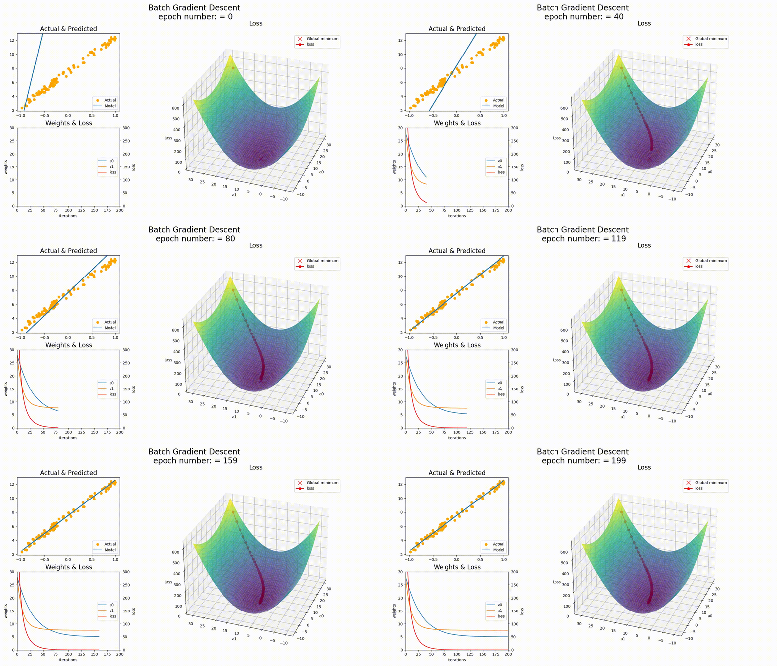
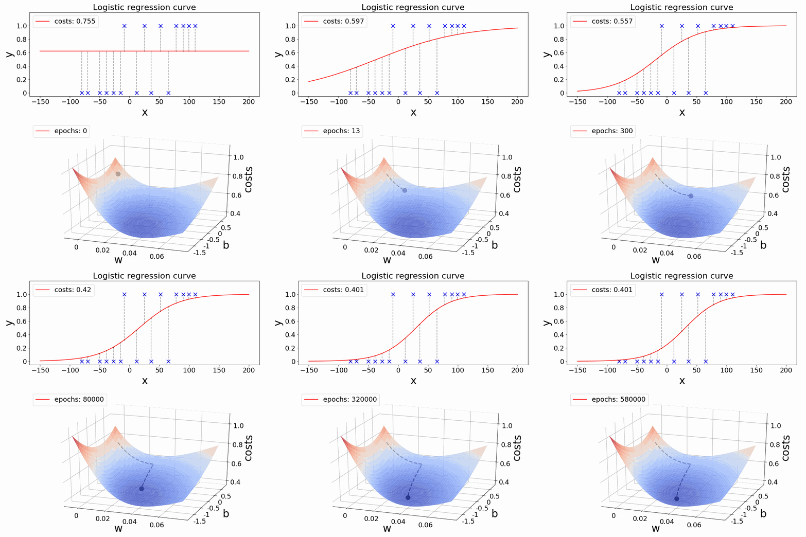
Here you are : — Now just observe the below two examples for Linear & Logistic Regression and observe the shape of line and global minima points simultaneously.

Nutshell, so far :-

Step 1: Define the Function

Define the function f ( Loss ) that we want to optimize.

cost = f(coefficient)

Step 2: Initialise Parameters

Initialize the parameters ( weights ) are usually set to random values.

These could be, coefficient = 0.0

Step 3: Compute the Gradient — Calculating the partial derivatives

For example, if we have a function f(x,y),

the gradient ∇f would be a vector containing ∂x / ∂f and ∂y / ∂f

delta = derivative(cost)

Step 4: Update Parameters

Move in the opposite direction of the gradient to minimize the function.

coefficient = coefficient — (alpha * delta), alpha — Learning rate.

Mathematically, the parameter update rule is often expressed as:

θ_new = θ_old − α ⋅ ∇f

where:

θ_old is the current value of the parameters.
α is the learning rate, which controls the size of the steps we take during optimization.
∇f is the gradient of the function for the parameters.

Step 5: Repeat Until Convergence

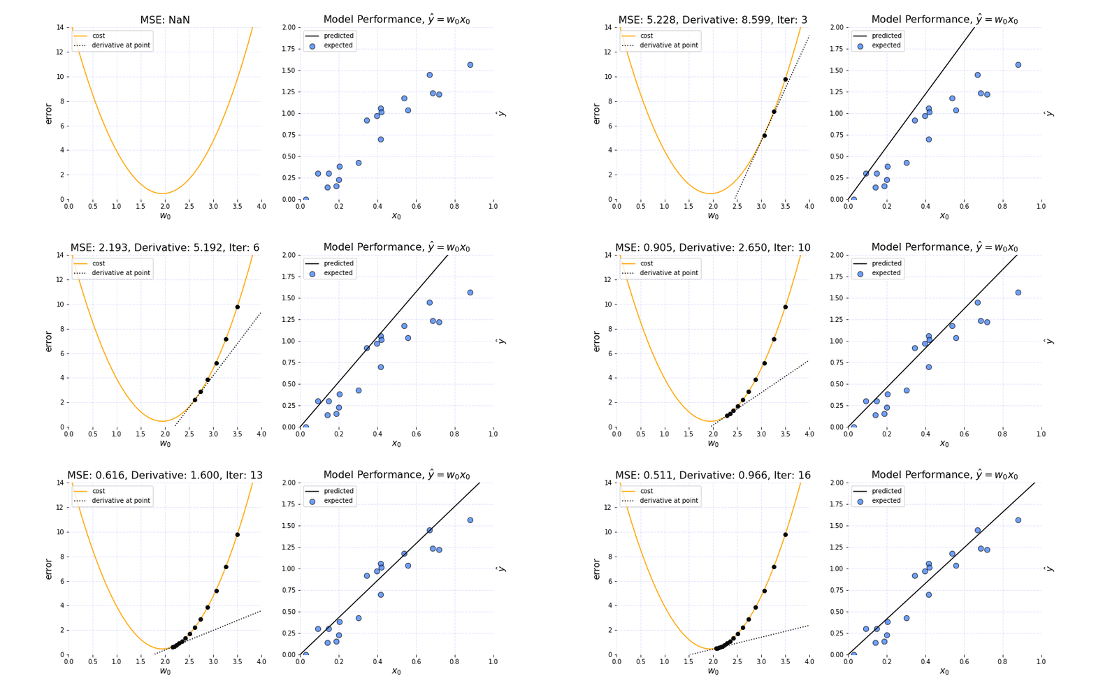
We iterate through steps 3 and 4 until a stopping criterion is met, such as reaching a specified number of iterations or achieving a certain level of convergence. During each iteration, we compute the gradient and update the parameters to gradually minimize the function.

Repeat until slope =0

Step 6: Evaluate Convergence

Finally, we evaluate the convergence of the optimization process by monitoring the value of the objective function or other performance metrics. If the optimization algorithm converges, we can consider the process complete and use the optimized parameters for inference or further analysis.

Learning rate — How fast weights Change

The learning rate is the size of the step, which dictates how quickly the algorithm converges or in other words how quickly the algorithm reaches global minima where the error is least.

The learning rate is denoted by the “Greek letter eta (η).” It is a positive scalar value typically ranging between 0.0 and 1.0. The most important hyper-parameters to tune for training deep neural networks.

How do we Decide ?

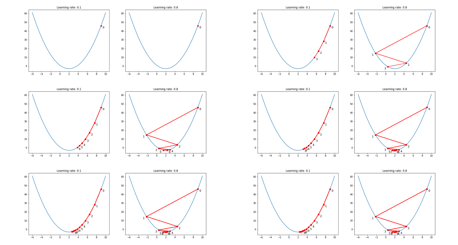
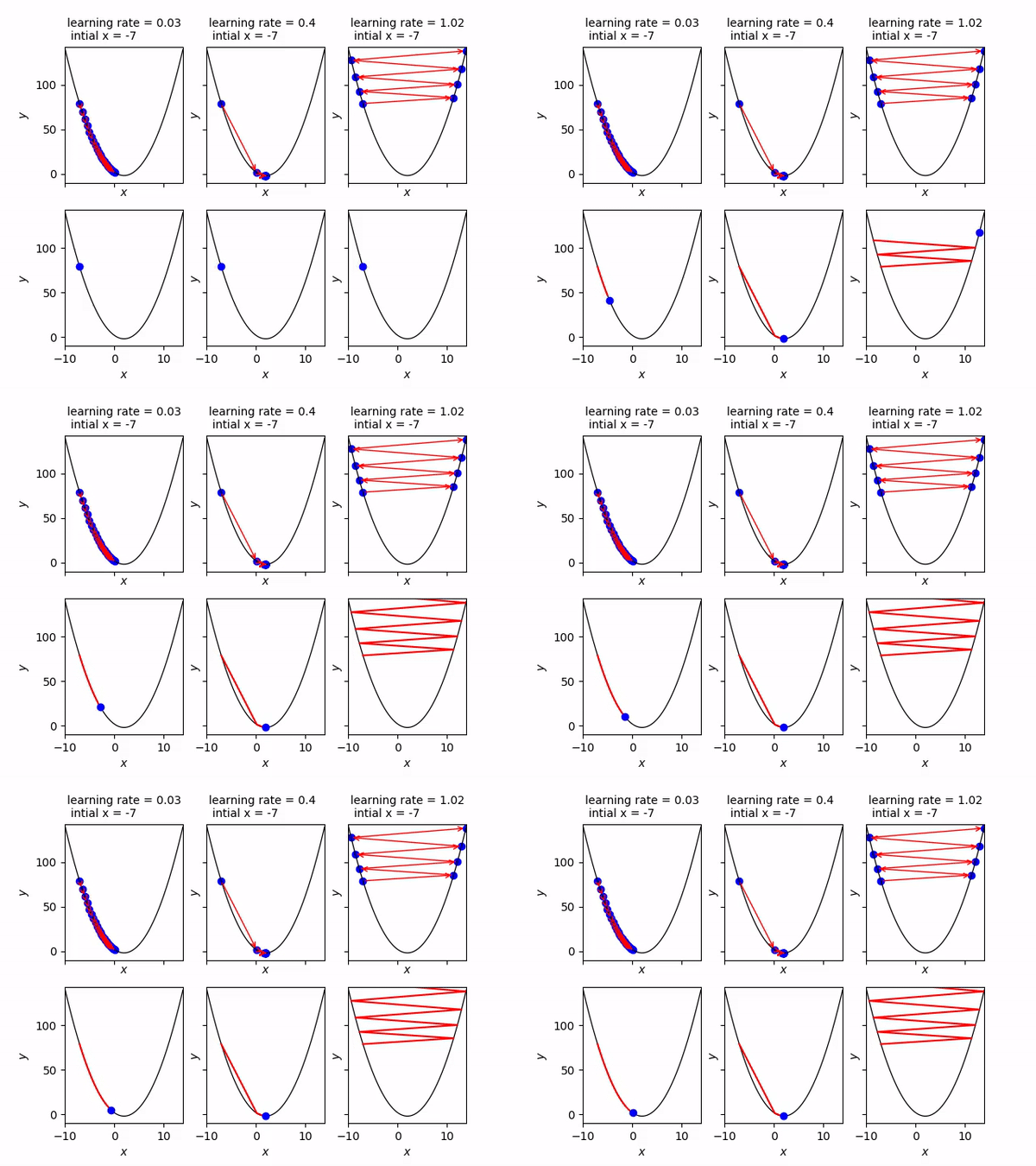
It is set by a matter of experimentation (usually small — e.g. 0.1) and tells how far to move. A learning rate of 0.1, a traditionally common default value, would mean that weights in the network are updated 0.1 * (estimated weight error) or 10% of the estimated weight error each time the weights are updated.The smaller the rate the longer it will take to reach the minima, or the lower the value, the slower we travel along the downward slope.The larger the rate the higher the risk of skipping the minima, or with a high learning rate we can cover more ground each step, but we risk overshooting the lowest point since the slope of the hill is constantly changing.

Choosing the Right Learning Rate:

Too High: If the learning rate is too high, you might overshoot the minimum and fail to converge.
Too Low: If it’s too low, the model might take tiny steps, making the training process extremely slow, or it might get stuck in a local minimum
Just Right: The challenge is finding a learning rate that’s just right — neither too high nor too low. Techniques like learning rate schedules or adaptive learning rate methods aim to address this challenge.

A good learning rate could be the difference between a model that doesn’t learn anything and a model that presents state-of-the-art results. The aim is to iterate this in order to find the global minimum.

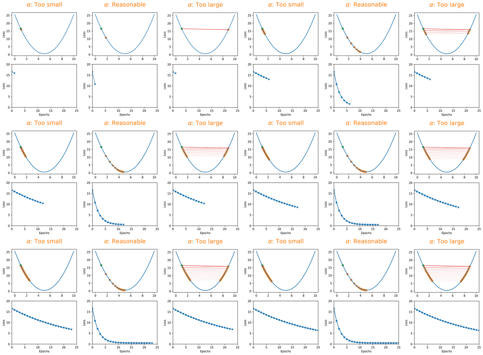
Hakuna Matata Meaning — Think of a simple function that has one number as input and one number as an output. The goal will be to start the input point and figure out in which direction to move in order to make the output lower. Learning rate determines how fast or slow we will move towards the optimal weights.

Challenges and Solutions

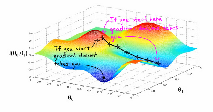
Local Minima: Gradient descent may converge to local minima instead of the global minimum, Adaptive learning rates (e.g., AdaGrad, RMSProp, Adam) can be the solutions.
Experimentation: It’s often a trial-and-error process to find the optimal learning rate. Start with a reasonable initial value and observe the behavior of the algorithm. If it converges too slowly, increase the learning rate; if it diverges or overshoots, decrease the learning rate. Iterate this process until you find the right balance or random restarts can also help mitigate this issue.
Learning Rate Selection: Choosing an appropriate learning rate is crucial for convergence. Techniques like learning rate schedules (e.g., exponential decay, step decay) and adaptive learning rate methods dynamically adjust the learning rate during optimization.
Feature Scaling: Gradient descent may converge slowly or fail to converge if features are not scaled properly. Standardization (mean normalization) or normalization (scaling to a range) can help alleviate this problem.
Cross-validation: Another method is to use a grid or random search to try different hyperparameters, including the learning rate, and pick the best combination based on cross-validation performance.
Using the below techniques may also solve the problem.

The most important thing is to be patient when optimizing gradient descent and optimizing gradient descent is an art, not a science ’’ — Tarun Sachdeva

Types of Gradient Descent

Batch Gradient Descent — 1 training example per iteration

Batch Gradient Descent also called Vanilla gradient descent is the first basic type of gradient descent in which we use the complete dataset available to compute the gradient of cost function.

While this approach guarantees convergence to the global minimum for convex functions, it can be computationally expensive and slow for large datasets as it calculates the error for each example within the training set. After it evaluates all training examples, it updates the model parameters. This process is often referred to as a training epoch.

Batch gradient descent uses the entire dataset to calculate each iteration of gradient descent

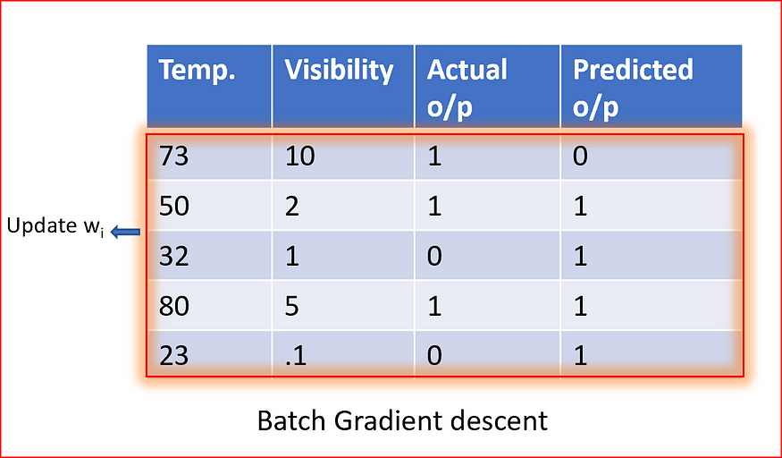
Stochastic Gradient Descent (SGD) — Used in Neural NetworkIn stochastic gradient descent, we use a single data point or example to calculate the gradient and update the weights with every iteration. This reduces computation time per iteration but introduces more variance in the parameter updates. Random sampling helps to arrive at a global minimum and avoids getting stuck at local minima.

We first need to shuffle the dataset so that we get a completely randomized dataset. As the dataset is randomized and weights are updated for every single example, the update of the weights and the cost function will be noisy jumping all over the place as shown below

Learning is much faster and convergence is quick for a very large dataset. There are many variations of stochastic gradient descent: Adam, RMSProp, and Adagrad.3. Mini-Batch Gradient Descent — Widely usedMini-batch gradient is a variation of stochastic gradient descent where instead of a single training example, a mini-batch of samples is used.

Mini-batch gradient descent strikes a balance between batch and stochastic gradient descent by updating the parameters using a small random subset of the dataset. It combines the advantages of both approaches, offering faster convergence and reduced variance.

All in All,

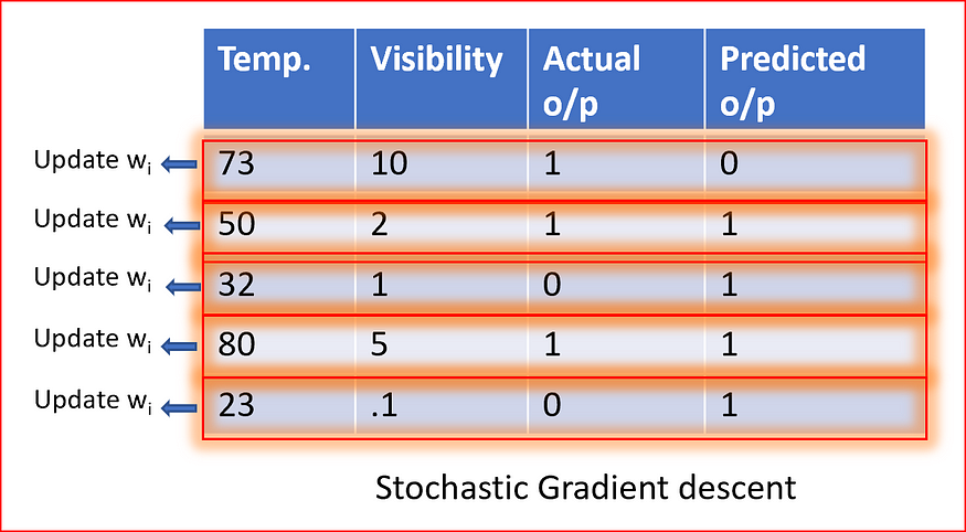
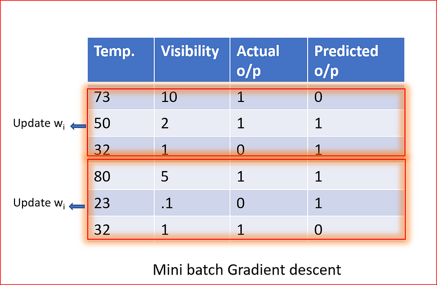
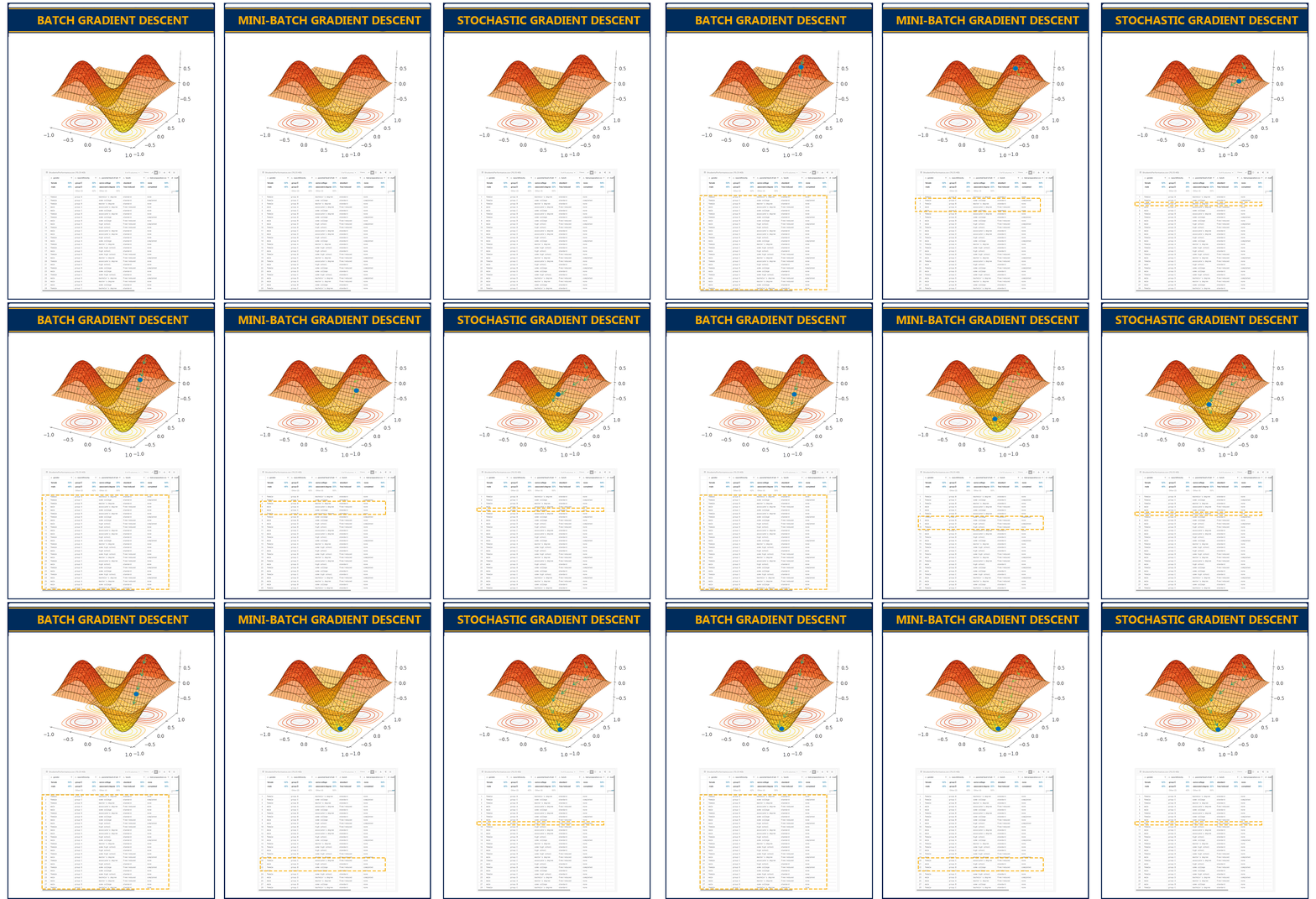
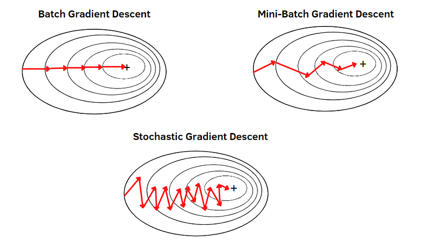
If the dataset is small (less than 2000 examples) use batch gradient descent. For larger datasets, typical mini-batch sizes are 64, 128, 256, or 512.

See the fluctuations of learning rate as well,

Don’t be afraid to try different things when optimizing gradient descent.” — Geoffrey Hinton

Hakuna Matata — Do not worry, just read this. 👍

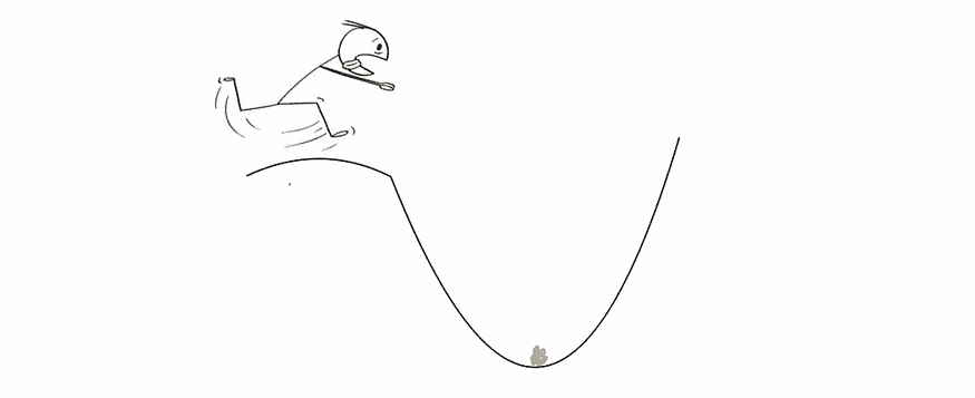
Let’s imagine you’re climbing down a mountain blindfolded and your goal is to reach the lowest point. Gradient Descent is like a savvy hiker finding the fastest way down a mountain.

Image Source — Tarun Sachdeva at **Gurudongmar Lake, Sikkim ( Near China ) —** 5,425 meters

Here’s how this scenario aligns with Gradient Descent:

The Mountain: Think of the landscape as a mathematical function with peaks and valleys. Your goal is to find the lowest point, which represents the minimum of the function.

Your Position: At any given moment, you are at a certain position on the mountain, but you can’t see the landscape around you due to the blindfold. This position corresponds to the current values of the parameters in the function you’re trying to optimize. In a nutshell, the Starting Point will begin randomly on the hill.

Direction: You want to descend the mountain efficiently. But without being able to see, you can only rely on your senses to feel the slope beneath your feet. The direction you choose to step in corresponds to the negative gradient of the function at your current position. If the slope is steeper in front of you, you take larger steps; if it’s gentler, you take smaller steps. In a nutshell, Feel the slope at your feet. Head downhill (steepest descent).

Step Size: The size of your steps corresponds to the learning rate in Gradient Descent. It determines how far you move in each direction. If the slope is steep, you might want to take larger steps to quickly descend, but if it’s too large, you risk overshooting the minimum. Conversely, if the slope is gentle, smaller steps might be more appropriate to avoid overshooting or oscillating around the minimum. In a nutshell, mind the steps not too big nor too small 👀

Iterative Process: You keep taking steps downhill, iteratively updating your position based on the slope of the terrain, until you reach a point where every step you take doesn’t get you any lower. This is analogous to reaching the bottom of the valley, where the gradient (slope) becomes nearly flat. In a nutshell, Take steps based on the slope until you reach the lowest point.

Convergence: Eventually, after many steps, you hope to reach the lowest point, which is the minimum of the function. This is your goal in the optimization process. However, in reality, you may stop before reaching the absolute minimum due to computational constraints or other considerations. 👌

You can think this way too, Imagine you’re at the top of a mountain range, and your goal is to find the most scenic spot, which offers the best panoramic view.

In essence, the learning rate is like deciding how big of a step you want to take while exploring a hilly terrain to find the lowest point. Too big, and you might jump over the lowest point; too small, and you might take forever to reach it. For challenges, Local minima, there might be many lowest points of the same terrain. In the world of data and AI, it’s a smart algorithm helping machines learn and optimize, finding the best path to minimize errors. 🏞️💻

It seems simple, but in real-time the terrain will look like this.😳