In Life & Statistics, everything is going to be normally distributed 😎

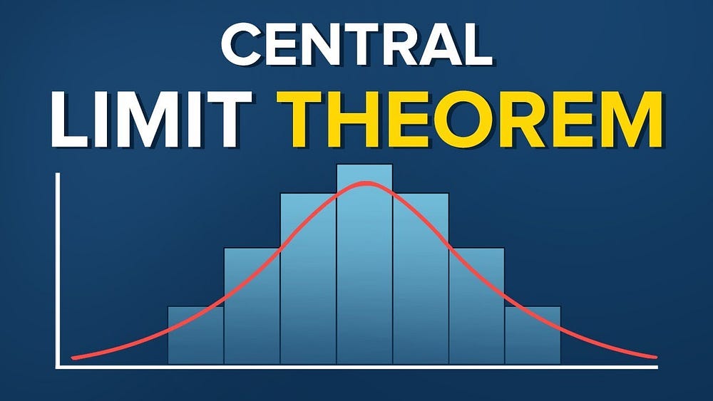
Have you ever wondered why certain patterns seem to emerge in everyday life, even when things seem random? Enter the Central Limit Theorem (CLT), a powerful concept in statistics that helps us make sense of the world around us.

The Central Limit Theorem (CLT) is a foundational concept in statistics, as it justifies why many statistical techniques rely on the assumption of normally distributed data.

The Central Ideas

The Central Limit Theorem can be summarized as :

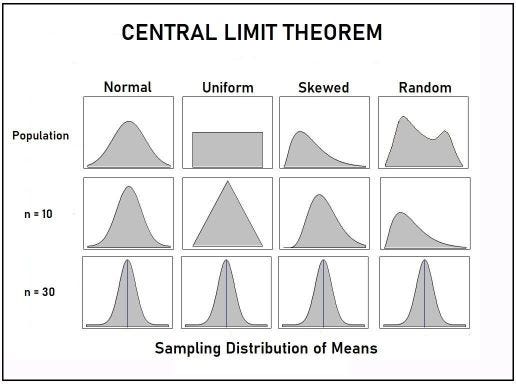
Given a sufficiently large sample size (n) drawn from any population with a mean (μ) and variance (σ²), the distribution of the sample mean (x̄) will approach a normal distribution, regardless of the shape of the original population distribution.

*except for the Cauchy Distribution, but let’s just ignore that.

In simple words, the central limit theorem states that if you take sufficiently large samples from a population, the sample mean will be normally distributed, even if the population isn’t normally distributed.

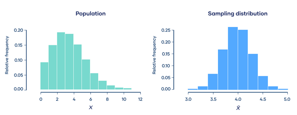
Explanation:- A population follows a Poisson distribution (left image). If we take 10,000 samples from the population, each with a sample size of 50, the sample means follow a normal distribution, as predicted by the central limit theorem.

The distribution of all sample statistics above is nearly normal, centered at the population mean, even though the population isn’t normally distributed.

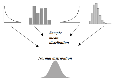
This is serious stuff, so let me reiterate one more time  — Maths behind

Numerically, means of random samples drawn from any population distribution with mean µ and standard deviation σ will have an approximately normal distribution with a mean equal to µ and standard deviation of σ /√n.

• The mean of the sampling distribution is the mean of the population.

• The standard deviation of the sampling distribution is the standard deviation of the population divided by the square root of the sample size.

We can describe the sampling distribution of the mean using this notation:

Where:

• X̄ is the sampling distribution of the sample means
• ~ means “follows the distribution”
• N is the normal distribution
• µ is the mean of the population
• σ is the standard deviation of the population
• n is the sample size

Sample size and standard deviations

The sample size affects the standard deviation of the sampling distribution. Standard deviation is a measure of the variability or spread of the distribution (i.e., how wide or narrow it is).

• When n is low, the standard deviation is high. There’s a lot of spread in the samples’ means because they aren’t precise estimates of the population’s mean.
• When n is high, the standard deviation is low. There’s not much spread in the samples’ means because they’re precise estimates of the population’s mean.

Distribution with Sample Size ( N )= 50

Distribution with Sample Size ( N )= 3

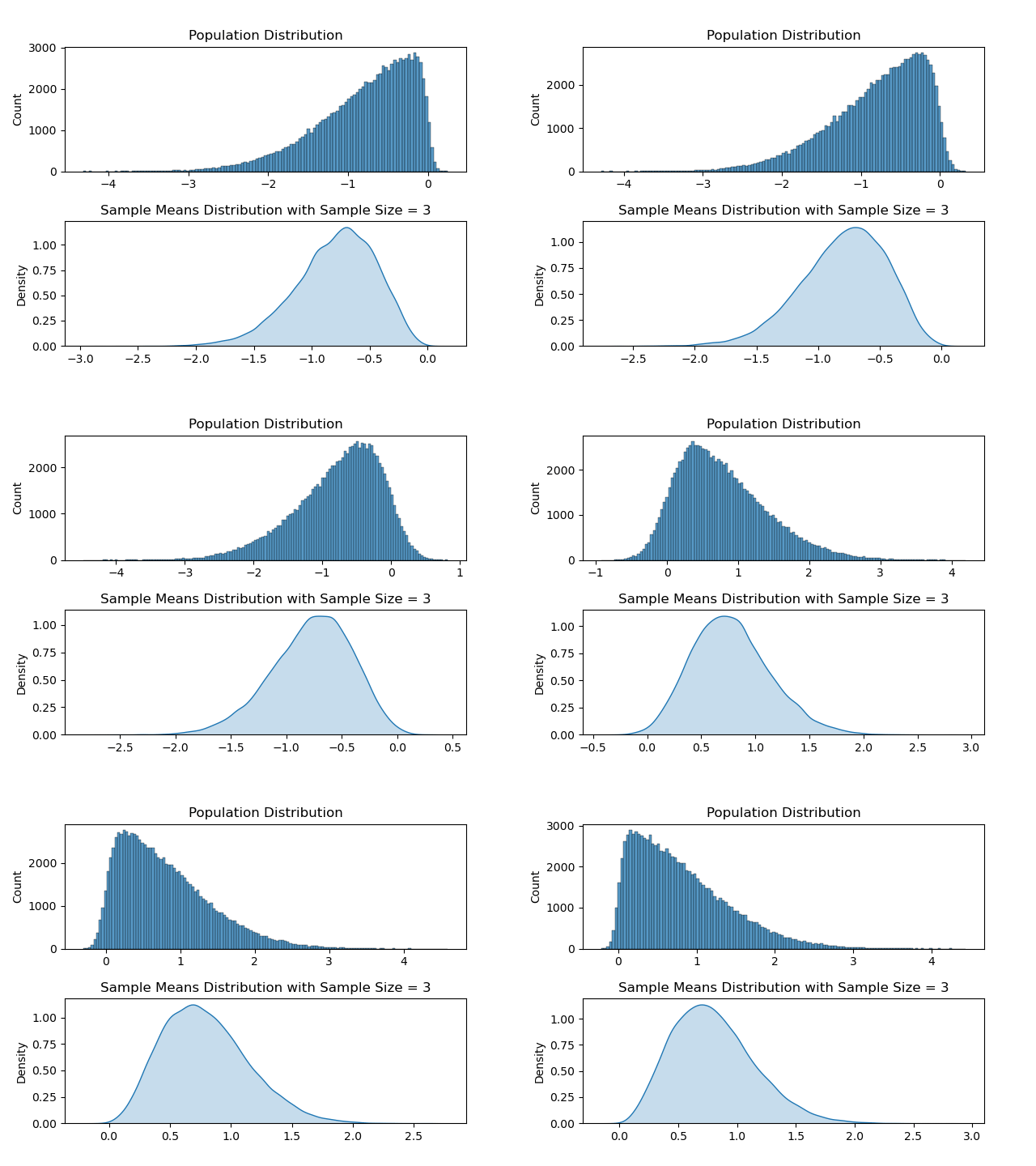
Hakuna Matata meaning when we add up lots of random things, like measurements or observations, the total tends to follow a predictable pattern, regardless of the shape of the original data.

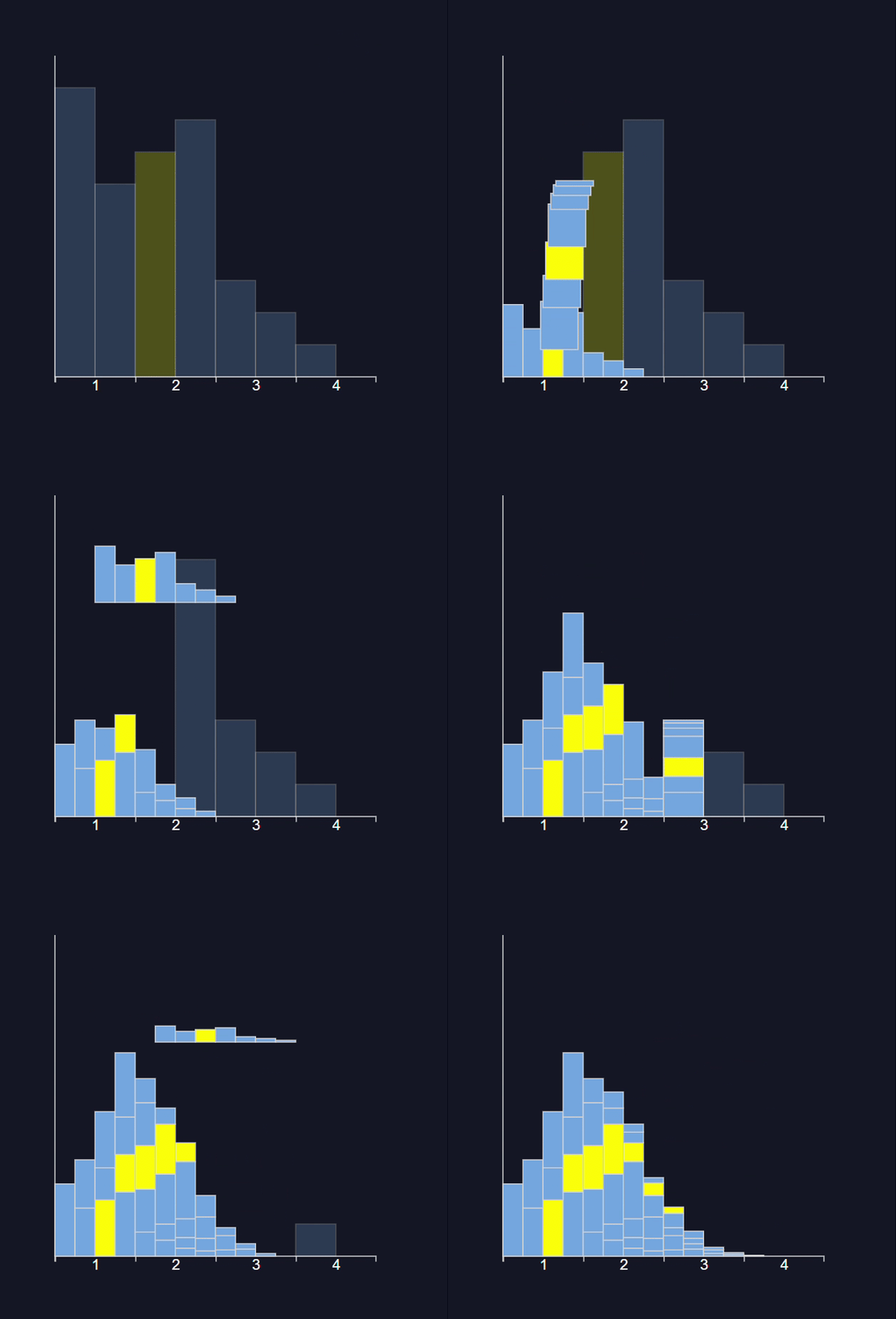
Easy Peasy No Problem — I am here to help you with Example.

Consider the game of tossing a coin. Every time the coin is tossed, make a note of it. Say the coin is tossed 100 times.

The result of each toss is noted as follows :

S = {H , T, T, T, H, H, T, H, H, T, T, H, H, T, T, T, H, T, H, H, T, H, T, H, H, T, H, H, H, T,T, T, H, T, T, T, H, H, T, H, T, H, H, T, T, H, H, T, T, T, H, T, H, T, H, T, H, H, T, T,H, H, T, T, H, H, T, H, T, T, H, H, T, H, H, T, T, H, T, H, H, T, H, T, T, T, H, T, H, T,T, H, T, H, H, T, T, H, T, H}

Let’s define a random variable as follows

X: Number of heads (H)

Draw random samples from S. Let the sample size (n) = 30 and S1, S2, S3, be three random samples drawn from S

S1: {H,H,T,H,T,T,T,H,T,H,T,H,H,T,H,H,T,T,H,T,T, T, H, H, T,T,T,H,T,H}

S2: { H,H,T,H,T,H,H,T,H,H,T,H,H,T,H,H,T,T,H,T,T,H,T,H,H,T,T,H,T,H }

S3: {T,T,H,T,T,T,H,H,T,H,T,H,H,T,T,H,H,T,T,T,T,H,H,T,H,H,T,T,H,T}

Compute the average number of times X is present in each of the samples

• S1: 14/30 = 0.46
• S2: 17/30 = 0.56
• S3: 13/30 = 0.43

Let’s plot these values!

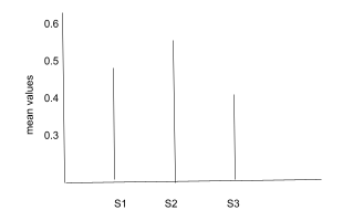
Hurrah! The distribution of the sample means approximately follows a normal distribution. 😄

See this now,

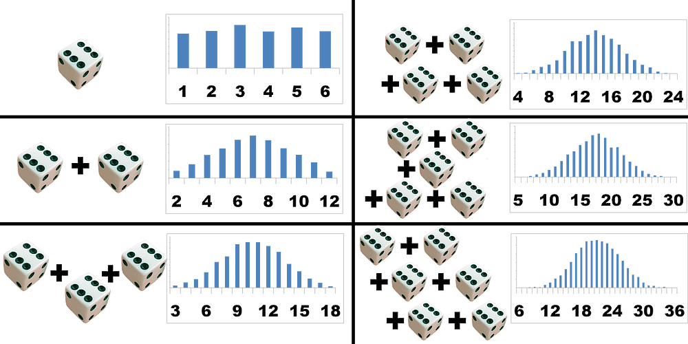
Read Again it takes time,

The Central Limit Theorem states that no matter how the distribution of the population is if I take a sufficiently large number of random samples (sample1, sample2, sample3, sample, and so on…) from the population and try to calculate the mean of sample’s and try to plot it then the sampling distribution of the sample mean will be normally distributed.

Historical Context

The story of the Central Limit Theorem begins in the early 19th century with the pioneering work of French mathematician Abraham de Moivre on the normal and binomial distribution.

He laid the groundwork for CLT with his studies on the distribution of the sum of independent random variables, particularly in the context of coin flips and dice rolls.

De Moivre was fascinated by games of chance, like dice rolling and coin flipping. He discovered that when you add up the outcomes of many independent events, the result tends to form a bell-shaped curve, now known as the normal distribution, and his work was published in 1733 as De Moivre’s Theorem.

Building on de Moivre’s work, another mathematician named Pierre-Simon Laplace refined the ideas behind CLT in the early 19th century with his work on the distribution of errors in astronomical observations.( Laplace distribution ) Laplace realized that this bell-shaped curve wasn’t just a curiosity; it was a fundamental property of randomness that could be applied to many different situations.

Carl Friedrich Gauss, commonly referred to as the “Prince of Mathematicians,” later played a significant role in advancing the study of normal distribution in the early 19th century. It was not until the early 20th century, with prominent statisticians such as Sir Ronald A. Fisher and Jerzy Neyman, that the CLT was formally stated and rigorously proven as It provides a precise statement about the convergence of the sample mean to a normal distribution as the sample size increases, regardless of the shape of the population distribution.

Rule of Thumb For Central Limit Theorem

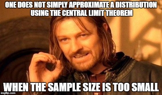
Generally, the Central Limit Theorem is used when the sample size is fairly big, usually larger than or equal to 30. In some cases even if the sample size is less than 30 central limit theory still holds but for this the population distribution should be close to normal or symmetric.

Breaking it Down: Why Does it Matter?

1. Understanding Randomness:

Randomness is all around us, from the outcomes of coin flips to the heights of people. CLT helps us understand how randomness behaves by showing that the total of many random things tends to follow a predictable pattern. Understanding CLT empowers us to navigate uncertainty confidently, finding order in life’s randomness.

2. Population Interference:

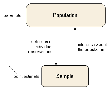
The field of statistics is based on the fact that it is highly impossible to collect data on the entire population. Instead of doing that we can gather a subset of data from a population and use the statistics of that sample to conclude the population.

3. Practical Applications:

• Imagine you’re flipping a coin multiple times. The more flips you do, the closer you get to a 50–50 split between heads and tails. That’s CLT in action, showing how patterns emerge from randomness with enough repetitions.

4. Everyday Examples:

• CLT influences various aspects of our lives, from predicting election outcomes to understanding test scores. It’s the reason why opinion polls can accurately predict election results and why test scores often form a bell curve.

5. By the 68–95–99 rule:-

1. 68% of the sample is within one standard deviation of the mean
2. 95% is within 2 standard deviations
3. 99.7% is within 3 standard deviations

The Central Limit Theorem (CLT) is like a magic wand that reveals hidden patterns in seemingly random data.

Here’s a fun demonstration of the CLT at work. In the bean machine or Galton Board, beads are dropped from the top and eventually accumulated in bins at the bottom in the shape of a bell curve.